SQL — Modeling, Queries, Data Quality & Pipeline
Educational examples on a fictitious e-commerce dataset (CH/EU), covering 2019–2024. The point is not to “show a stack”, but to highlight what you can actually do with SQL: build a simple model, produce readable KPIs, read an execution plan to optimize a query (sargable), validate data quality, and track a pipeline in lightweight production.
P1 — Modeling & Business Queries
Context & objectives
We start from a minimal relational model to illustrate what SQL can do:
clear queries, monthly indicators, and reusable results for a dashboard.
We rely on explicit types, primary/foreign keys, and simple constraints
(NOT NULL, CHECK).
On the query side, we combine CTEs (WITH) and a few
window functions (e.g. SUM() OVER) to aggregate properly.
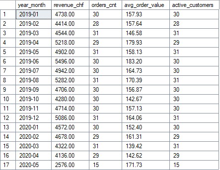
Target metrics: Revenue (CHF), number of orders,
average basket, and active customers per month.
Monthly KPIs (excerpt)
P2 — Performance & Indexing (Execution Plans)
The goal: rewrite a query to make it sargable (search-ARGument-able) and leverage a proper index. Here, the “Top customers by period” query applied a function on the date column, forcing the optimizer to scan more rows than necessary.

CONVERT(date, o.order_date)),
index cannot be used effectively → wide scan.
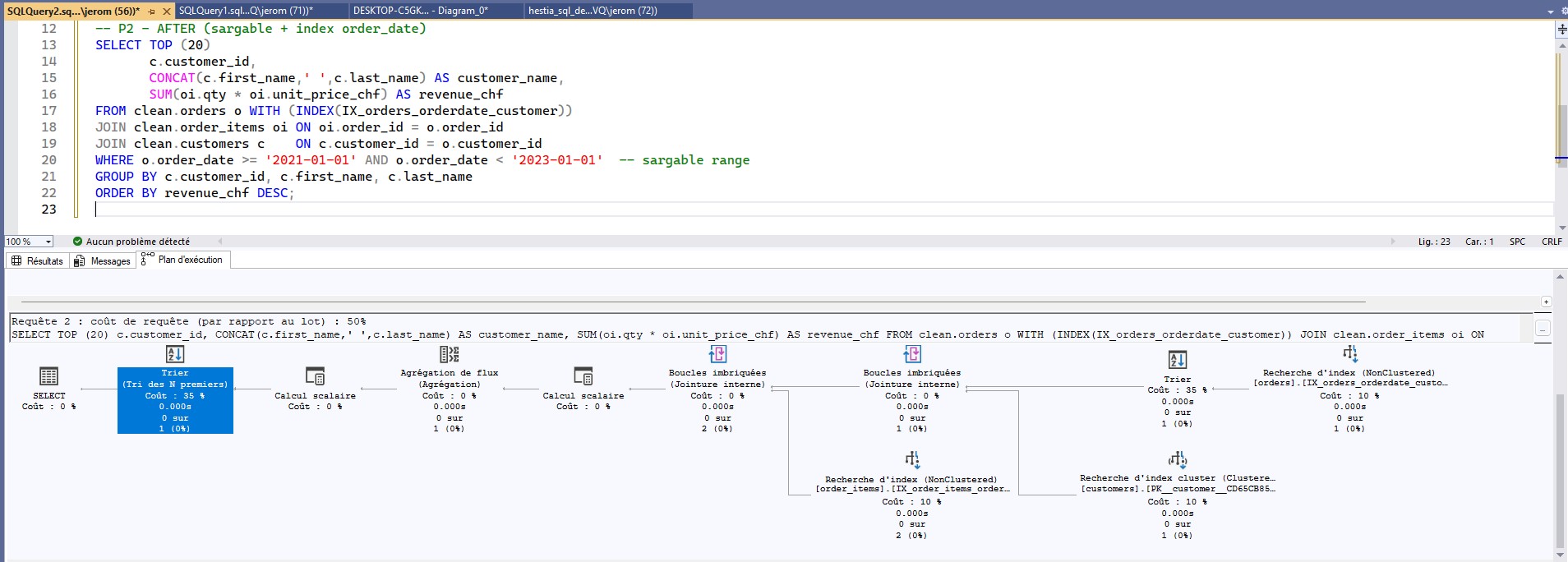
o.order_date >= '2021-01-01' AND o.order_date < '2023-01-01')
+ composite index (order_date, customer_id) → lighter plan, cheaper sort.
Best practices: limit selected columns, prefer EXISTS over
IN when appropriate, pre-aggregate if needed, and
read the plan (costs, operators).
P3 — Data Quality & Reliability
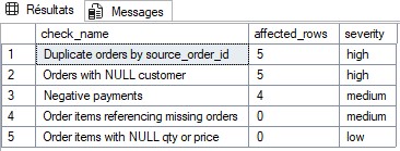
This illustrates what SQL can do to make datasets more reliable:
data quality rules (duplicates, NULL, orphan references, negative values),
consistent formatting, and prioritization of fixes.
A view consolidates results for dashboards or alerting systems.
- Simple rules (composite key uniqueness,
CHECKconstraints). - Severity-based prioritization to handle highest-impact issues first.
- Example corrections (safe
UPDATE/DELETE).
P4 — Lightweight ETL & Execution Log
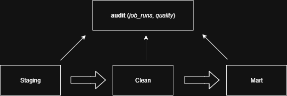
A “lightweight” SQL pipeline remains readable and idempotent: incremental loads, MERGE/UPSERT, technical keys, timestamps. Scheduling can be handled via CRON/Azure DevOps at 08:30 CET, with retries on failure.
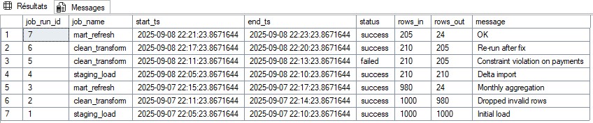
job_runs): start/end timestamps, status, rows_in/out, message.
Demo output: rerun after fix, constraint violation, delta import, monthly aggregation, etc.
Expected output: a simple, observable and traceable pipeline, ready to connect to an operational dashboard.